Fast Fourier Transform and Number Theoretic Transform

tl;dr: The Fast Fourier Transform (FFT) is generally credited to Cooley and Tukey in 1965, although its earliest ideas can be traced back to Gauss’s unpublished manuscript around 1805. FFT is one of the foundational algorithms behind modern high-performance computation: it accelerates integer multiplication and polynomial multiplication, and was named by IEEE as one of the top ten algorithms of the twentieth century. Current NIST post-quantum standards such as Kyber, Dilithium, and Falcon all involve FFT and its finite-field analogue, the Number Theoretic Transform (NTT). In addition, NTT is a critical acceleration primitive in practical zero-knowledge proof systems such as Plonk and in fully homomorphic encryption schemes such as BFV and TFHE. This article explains the mathematical theory and practical value of FFT and NTT in detail.

Disclaimer: This article is the English counterpart automatically generated from the original Chinese blog by Codex + GPT-5. The translation aims to preserve the original meaning, structure, and technical details as faithfully as possible. If there is any ambiguity or inaccuracy, please refer to the original Chinese version.

---

Discrete Fourier Transform

Let an \(n-1\) degree polynomial be written as

\[A(x) = a_0 x^0 + a_1 x^1 + \dots + a_{n-1} x^{n-1}\]

In particular, we assume that the polynomial degree bound, or equivalently the length of the coefficient vector, is \(n = 2^k\). In the non-power-of-two case, we can pad the higher-degree coefficients with zeros until the coefficient-vector length becomes a power of two. Let the \(n\)-th roots of unity be \(w_{n,k} = e^{\frac{2 k \pi i }{n}}\), where \(k \in [0..n-1]\), and let the primitive root of unity be \(w_{n} = w_{n, 1} = e^{\frac{2 \pi i }{n}}\). They all satisfy \(x^n = 1\).

The coefficient-vector representation of a polynomial is the most common one, namely \(\vec{A} = (a_0, a_1, \ldots, a_{n-1})\) above. The discrete Fourier transform is a special evaluation representation: it represents the polynomial as a vector of evaluations at the special \(n\)-th roots of unity:

\[\begin{aligned} \hat{A} &= \mathsf{DFT}(\vec A) = \mathsf{DFT}(a_0, a_1, \dots, a_{n-1})\\ &= (A(w_{n, 0}), A(w_{n, 1}), \dots, A(w_{n, n-1})) \\ &= (A(w_n^0), A(w_n^1), \dots, A(w_n^{n-1})) \\ &:= (y_0, y_1, \dots, y_{n-1}) \\ \end{aligned}\]

The inverse discrete Fourier transform essentially converts the evaluation representation of a polynomial back into the usual coefficient-vector form. This transformation is also better known as Lagrange interpolation for polynomials. Thus, the (inverse) discrete Fourier transform is an algorithm for converting between these two representations, namely the following maps:

\[\begin{cases} \mathsf{DFT}_{n}: \underbrace{(a_0, a_1, \ldots, a_{n-1})}_{\text{coefficient form}} \mapsto \underbrace{(y_0, y_1, \ldots, y_{n-1})}_{\text{evaluation form}} \\ \mathsf{iDFT}_{n}: \underbrace{(y_0, y_1, \ldots, y_{n-1})}_{\text{evaluation form}} \mapsto \underbrace{(a_0, a_1, \ldots, a_{n-1})}_{\text{coefficient form}} \\ \end{cases}\]

Convolution and Fourier Transform

In communications, the Fourier transform (Continuous Time Fourier Transform) is usually a powerful tool for studying continuous signals. It converts continuous time-domain information into frequency information, or a spectrum:

\[S(f) = \int_{-\infty}^{\infty} s(t) \cdot e^{-i2\pi ft} \, dt\]

On existing computers, however, it is impossible to simulate a fully continuous time-domain signal. Therefore, the discrete Fourier transform has greater practical value, and this leads naturally to the discrete-time Fourier transform.

1. Discrete Fourier Transform (DFT) converts a sequence of complex numbers \(\{x_n\} := x_0, x_1, \dots, x_{N-1}\) into another sequence of complex numbers of the same length \(\{X_k\} := X_0, X_1, \dots, X_{N-1}\). Its forward transform is mathematically defined as follows:

   \[X_k = \sum_{n=0}^{N-1} x_n \cdot e^{-i 2\pi \frac{k}{N} n}, \quad k = 0, \dots, N-1\]

   Here \(x_n\) is the sampled signal in the time domain, \(X_k\) is the frequency component in the frequency domain, and \(N\) is the sequence length. The term \(e^{-i 2\pi \frac{k}{N} n}\) is the complex exponential basis function, which can be expanded by Euler’s formula as \(\cos(2\pi \frac{k}{N} n) - i \sin(2\pi \frac{k}{N} n)\).

2. Inverse Discrete Fourier Transform (Inverse DFT) recovers the time-domain sequence from the frequency-domain sequence:

   \[x_n = \frac{1}{N} \sum_{k=0}^{N-1} X_k \cdot e^{i 2\pi \frac{k}{N} n}, \quad n = 0, \dots, N-1\]

   Note that signal-processing conventions usually use a negative exponent for the forward DFT, whereas this article uses a positive exponent convention from the polynomial-evaluation perspective: \(y_k=\sum_{j=0}^{n-1}a_j w_n^{kj}\). The two directions are conjugate to each other; what matters is that the forward and inverse transforms are used consistently.

Switching back to the polynomial perspective, we obtain the following somewhat imprecise analogy:

Time-domain representation	After the discrete Fourier transform	Practical meaning of the Fourier transform
Continuous time-domain signal of a wave	Spectrum information (frequency, amplitude, phase)	Frequency decomposition and component analysis of waves: decompose a superposition of waves into sinusoidal waves of single frequencies, making it easier to compute superposition and spectrum information
Coefficient vector of a polynomial	Evaluation form of the polynomial	Accelerating polynomial multiplication: by analogy with wave superposition, it enables fast convolution, i.e. multiplication

In essence, convolution and multiplication are equivalent: multiplying two polynomials is essentially taking the linear convolution of their coefficient sequences. To make the later discussion of NTT more convenient, we directly consider the integer quotient ring \(\mathbb{Z}_q[x]\) here.

It is easy to verify that the linear convolution above is equivalent to polynomial multiplication. After a polynomial is transformed into its evaluation form by the discrete Fourier transform, convolution operations become more convenient. Beyond linear convolution, cryptography often uses cyclic convolution:

• Positive wrapped convolution (PWC): equivalent to multiplication in the polynomial quotient ring \(\mathbb{Z}_q[x] / (x^n - 1)\)
• Negative wrapped convolution (NWC): equivalent to multiplication in the polynomial quotient ring \(\mathbb{Z}_q[x] / (x^n + 1)\)

Negacyclic convolution, also often called Negative Wrapped Convolution (NWC), is one of the core acceleration operations in lattice-based cryptography such as Kyber and Dilithium, as well as in fully homomorphic encryption.

Fast Fourier Transform

How can we implement \(\mathcal{O}(n \log n)\) algorithms for \(\mathsf{DFT}\) and \(\mathsf{iDFT}\)? We know that ordinary point evaluation costs \(\mathcal{O}(n)\), so the naive \(\mathsf{DFT}\) has complexity \(\mathcal{O}(n^2)\). The naive Lagrange interpolation algorithm also has complexity \(\mathcal{O}(n^2)\). The core of the Fast Fourier Transform lies in the special root-of-unity basis vector used by the evaluation representation:

\[\vec w = (w_{n,0}, w_{n,1}, \ldots, w_{n,n-1}) = (w_n^0, w_n^1, \ldots, w_n^{n-1})\]

The central algorithmic idea is divide and conquer. We know that:

\[\begin{aligned} A(x) &= a_0 x^0 + a_1 x^1 + \dots + a_{n-1} x^{n-1} \\ &= a_0 x^0 + a_2 x^2 + \dots + a_{n-2} x^{n-2} + x(a_1 x^0 + a_3 x^2 + \dots + a_{n-1}x^{n-2}) \\ &= A_0(x^2) + xA_1(x^2) \end{aligned}\]

Here \(A_0(x), A_1(x)\) are both polynomials with only \(\frac{n}{2}\) coefficients, satisfying:

\[\begin{aligned} A_0(x) &= a_0 x^0 + a_2 x^1 + \dots + a_{n-2} x^{\frac{n}{2}-1} \\ A_1(x) &= a_1 x^0 + a_3 x^1 + \dots + a_{n-1} x^{\frac{n}{2}-1} \end{aligned}\]

DFT Algorithm \(\mathcal{O}(n \log n)\)

Let \(T_{\mathsf{DFT}}(n)\) denote the time complexity of computing the discrete Fourier transform of a degree-\(n\) polynomial. From the decomposition \(A(x) = A_0(x^2) + xA_1(x^2)\), if we can obtain the \(\mathsf{DFT}\) vector of \(A\) in \(O(n)\) time from the known \(\mathsf{DFT}\) vectors of \(A_0\) and \(A_1\), then the complexity satisfies the following recurrence:

\[T_{\mathsf{DFT}}(n) = 2T_{\mathsf{DFT}}(\frac{n}{2}) + \mathcal{O}(n)\]

By the Master theorem for recurrences, the final time complexity of this recursive algorithm is \(\mathcal{O}(n \log n)\). A key observation is that squaring the vector of \(n\)-th roots of unity, \(\vec w^2 = (w_n^0, w_n^2, \ldots, w_n^{2(n-1)})\), gives exactly all \(\frac{n}{2}\)-th roots of unity. Therefore, the input pattern in the evaluation representations of \(A_0(x)\) and \(A_1(x)\) matches that of \(A(x)\) precisely. More concretely, suppose we already know \(A_0(x), A_1(x)\) and their discrete Fourier transforms:

\[\begin{cases} \left(y_k^0\right)_{k=0}^{n/2-1} = \mathsf{DFT}(A_0) \\ \left(y_k^1\right)_{k=0}^{n/2-1} = \mathsf{DFT}(A_1) \end{cases}\]

Using the special properties of roots of unity:

\[\begin{cases} w_{n}^{2k} = e^{\frac{2\pi k i}{n/2}} = w_{n/2}^{k} & k \in [0, n/2 - 1] \\ w_{n}^{k + \frac{n}{2}}= - w_{n}^{k} & k \in [0, n - 1] \end{cases}\]

Therefore, the \(n\) evaluation values of \(\mathsf{DFT}(A)\) can be recovered as follows:

\[\begin{cases} y_k = A_0(w_n^{2k}) + w_n^{k} \cdot A_1(w_n^{2k}) = y_k^0 + w_n^k y_k^1, & k = 0, \ldots, \frac{n}{2} - 1. \\ y_k = A_0(w_n^{2k}) + w_n^{k} \cdot A_1(w_n^{2k}) = y_{k \bmod \frac{n}{2}}^{0} + w_n^{k} y_{k \bmod \frac{n}{2}}^{1} & k = \frac{n}{2}, \ldots, {n} - 1. \\ \end{cases}\]

Written more elegantly:

\[\begin{cases} y_k &= y_k^0 + w_n^k y_k^1, &\quad k = 0 \dots \frac{n}{2} - 1, \\ y_{k+n/2} &= y_k^0 - w_n^k y_k^1, &\quad k = 0 \dots \frac{n}{2} - 1. \end{cases}\]

This formula is also called the butterfly formula. The whole recursive expression is quite elegant: using the butterfly formula, one only needs \(\mathcal{O}(n)\) time to recover the DFT of \(A\) from the DFTs of \(A_0\) and \(A_1\). In summary, we have obtained a recursive \(\mathcal{O}(n \log n)\) algorithm for the discrete Fourier transform \(\mathsf{DFT}\).

iDFT Algorithm \(\mathcal{O}(n \log n)\)

Simply put, this is polynomial interpolation. Lagrange interpolation can compute it in \(\mathcal{O}(n^2)\) time. Essentially, this is solving a system of linear equations:

\[\underbrace{ \begin{pmatrix} w_n^0 & w_n^0 & w_n^0 & w_n^0 & \cdots & w_n^0 \\ w_n^0 & w_n^1 & w_n^2 & w_n^3 & \cdots & w_n^{n-1} \\ w_n^0 & w_n^2 & w_n^4 & w_n^6 & \cdots & w_n^{2(n-1)} \\ w_n^0 & w_n^3 & w_n^6 & w_n^9 & \cdots & w_n^{3(n-1)} \\ \vdots & \vdots & \vdots & \vdots & \ddots & \vdots \\ w_n^0 & w_n^{n-1} & w_n^{2(n-1)} & w_n^{3(n-1)} & \cdots & w_n^{(n-1)(n-1)} \end{pmatrix} }_{\mathbf{V} \in \mathbb{C}^{n \times n}} \begin{pmatrix} a_0 \\ a_1 \\ a_2 \\ a_3 \\ \vdots \\ a_{n-1} \end{pmatrix} = \begin{pmatrix} y_0 \\ y_1 \\ y_2 \\ y_3 \\ \vdots \\ y_{n-1} \end{pmatrix}\]

Here \(\mathbf{V} \in \mathbb{C}^{n \times n}\) is the Vandermonde matrix. Its inverse is:

\[\mathbf{V}^{-1} = \frac{1}{n} \begin{pmatrix} w_n^0 & w_n^0 & w_n^0 & w_n^0 & \cdots & w_n^0 \\ w_n^0 & w_n^{-1} & w_n^{-2} & w_n^{-3} & \cdots & w_n^{-(n-1)} \\ w_n^0 & w_n^{-2} & w_n^{-4} & w_n^{-6} & \cdots & w_n^{-2(n-1)} \\ w_n^0 & w_n^{-3} & w_n^{-6} & w_n^{-9} & \cdots & w_n^{-3(n-1)} \\ \vdots & \vdots & \vdots & \vdots & \ddots & \vdots \\ w_n^0 & w_n^{-(n-1)} & w_n^{-2(n-1)} & w_n^{-3(n-1)} & \cdots & w_n^{-(n-1)(n-1)} \end{pmatrix} \\ \implies \begin{pmatrix} a_0 \\ a_1 \\ a_2 \\ a_3 \\ \vdots \\ a_{n-1} \end{pmatrix} = \mathbf{V}^{-1} \begin{pmatrix} y_0 \\ y_1 \\ y_2 \\ y_3 \\ \vdots \\ y_{n-1} \end{pmatrix}\]

Therefore, the Lagrange interpolation formula in this special form is also very elegant. We can directly express \(a_{k}\) in polynomial form as:

\[a_k = \frac{1}{n} \sum_{j=0}^{n-1} y_j w_n^{-k j}\]

This gives us a problem almost identical to the expression \(y_k = \sum_{j=0}^{n-1} a_j w_n^{k j}\) for \(\mathsf{DFT}\). The key changes are:

\[\begin{cases} 1 &\implies \frac{1}{n} \\ w_n^{k j} &\implies w_n^{-k j} \end{cases}\]

The recursive algorithm from the previous section applies equally well in this setting. In summary, we have obtained a recursive \(\mathcal{O}(n \log n)\) algorithm for the inverse discrete Fourier transform \(\textsf{iDFT}\).

The core of FFT acceleration: The fundamental reason FFT is fast is the periodicity of roots of unity:

\[w_{n}^{n} = 1, \quad w_{n}^{\frac{n}{2}} = -1\]

This allows many computations to be reused, which is the essence of the recursive acceleration. In the later discussion of NTT, we will further explain how to reuse computation through the periodicity of roots of unity.

Fast Number Theoretic Transform

In cryptography, we usually care about polynomials over integer rings. More specifically, we care about polynomials over the integer quotient ring \(\mathbb{Z}_{q}\), and in most cases we regard \(q\) as a prime. In this section, all multiplication operations are explained through convolution, namely the following correspondence:

Linear Convolution	Cyclic Convolution / Positive Wrapped Convolution	Negacyclic Convolution
Multiplication in \(\mathbb{Z}_q[x]\)	Multiplication in \(\mathbb{Z}_q[x] / (x^n - 1)\)	Multiplication in \(\mathbb{Z}_q[x] / (x^n + 1)\)

Over integer quotient rings, we need to find a root of unity with the same properties as \(e^{\frac{2\pi i}{n}}\) in the discrete Fourier transform: the primitive root of unity over \(\mathbb{Z}_{q}\) defined below.

Linear / Positive Wrapped Convolution

It is easy to verify that the two matrices corresponding to the expressions above in \(\hat{\mathbf{a}}\) and \({\mathbf{a}}\) are inverses of each other:

\[\mathbf{a} = \textsf{iNTT}^{\omega}\left(\textsf{NTT}^{\omega}\left(\mathbf{a}\right)\right)\]

Thus, linear convolution can be computed via NTT as follows. Note that when computing linear convolution in \(\mathbb{Z}_q[x]\), one should choose a transform length \(m \ge 2n-1\) and zero-pad the input:

\[\mathbf{c} = \mathbf{a} * \mathbf{b} = \textsf{iNTT}^{\omega}\left(\textsf{NTT}^{\omega}\left(\mathbf{a}\right) \circ \textsf{NTT}^{\omega}\left(\mathbf{b}\right)\right)\]

The acceleration techniques from FFT can be transferred completely to NTT and iNTT. Earlier, we mentioned that if we want to compute linear convolution over \(\mathbb{Z}_q[x]\), the dimension of \(\mathbf{c}\) should be \(2n - 1\). If we only use an \(n\)-th primitive root of unity and a transform of length \(n\), then we do not obtain linear convolution, but cyclic convolution. At this point, switching to the polynomial perspective, the values obtained after convolution are still the genuine values of \(A(\omega^i) \cdot B(\omega^i) \bmod q\), but the coefficients of monomials of degree \(\ge n\) have been cyclically accumulated into lower-degree coefficients. Because we are using an \(n\)-th primitive root, it satisfies \(x^{n + k} = x^k\), which is equivalent to:

\[x^{n+k} \equiv x^k \pmod {x^{n} - 1}\]

That is, the result is reduced modulo the polynomial \({x^{n} - 1}\). In coefficient terms, the true higher-degree monomial coefficients are cyclically accumulated into lower-degree monomial coefficients, which is exactly the expression for positive wrapped convolution:

\[y_k = \sum_{i=0}^{k} g_i \cdot h_{k-i} + \sum_{i=k + 1}^{n-1} g_i \cdot h_{k + n - i}\]

Let \(\textsf{NTT}_{n}^{\omega}(\cdot)\) denote the number theoretic transform acting on an \(n\)-dimensional vector using the primitive generator \(\omega\). Unless otherwise specified, we omit the parameter \(n\) and assume it matches the actual vector dimension, writing it simply as \(\textsf{NTT}^{\omega}(\cdot)\). We then obtain the following proposition.

The more essential point is that the \(n\)-th primitive roots selected by NTT all satisfy:

\[x^n = 1 \iff x^n - 1= 0\]

Therefore, the final result is plainly equivalent to the result after reducing modulo the polynomial \(x^n - 1\). This gives a more intuitive understanding of PWC and also helps us understand the mathematical intuition behind NWC in the next section.

Negacyclic Convolution

Next, consider how to compute negacyclic convolution. From the expression

\[y_k = \sum_{i=0}^{k} g_i \cdot h_{k-i} - \sum_{i=k + 1}^{n-1} g_i \cdot h_{k + n - i}\]

we naturally think that coefficients of monomials of degree \(\ge n\) are also accumulated into the corresponding lower-degree terms after reducing degrees modulo \(n\), except that their contribution to the coefficients is negative. Thus, we naturally want the relation \(x^{n + k} = -x^{k}\). In other words, the primitive root \(\varphi\) for this NTT should satisfy \(\varphi^{n} = - 1\), so \(\varphi\) is a primitive \(2n\)-th root of unity. However, if we simply replace \(\omega\) in positive wrapped convolution by \(\varphi\), this does not directly produce negacyclic convolution; instead, it introduces a frequency shift or a mathematical mismatch. Moreover, the evolution of twiddle factors in the standard NTT is based on the primitive-root sequence \(\omega^0, \omega^1, \omega^2, \ldots, \omega^{n-1}\) satisfying \(x^n = 1\). If we simply replace it by \(\varphi^0, \varphi^1, \varphi^2, \ldots, \varphi^{n-1}\), then half of these \(2n\)-th roots of unity do not have a consistent identity of either \(x^n = 1\) or \(x^n = -1\), and this property is crucial for fast NTT. Here I give two mathematical ways to understand NWC constructions.

Let \(\varphi\) be a primitive \(2n\)-th root of unity, and let \(\omega\) be a primitive \(n\)-th root of unity satisfying \(\omega = \varphi^2\).

The two viewpoints above yield the same result. We obtain the formal definition of the negacyclic Number Theoretic Transform as follows.

Similarly, by inverting the Vandermonde matrix, we can obtain the formula for the inverse negacyclic Number Theoretic Transform. It is worth pointing out that the paper https://eprint.iacr.org/2024/585.pdf contains a major typo in its definition of iNTT.

It is easy to verify that the two matrices corresponding to the expressions above in \(\hat{\mathbf{a}}\) and \({\mathbf{a}}\) are inverses of each other:

\[\mathbf{a} = \textsf{iNTT}^\varphi \left(\textsf{NTT}^\varphi\left(\mathbf{a}\right)\right)\]

The Essence of the Number Theoretic Transform

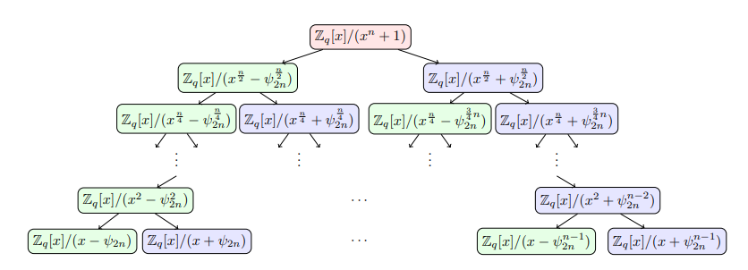
Returning to the algebraic perspective, the essence of the Number Theoretic Transform is ring decomposition and isomorphism. We take NWC as an example. Let \(\varphi\) be a primitive \(2n\)-th root of unity over \(\mathbb{Z}_q\). Then the cyclotomic polynomial \(C(X) = X^{n} + 1\) has the following factorization:

\[C(X) = \prod_{i=0}^{n-1} (X - \varphi^{2i + 1})\]

By the Chinese Remainder Theorem, there is a ring isomorphism:

\[\mathbb{Z}_q[X] / (X^n + 1) \cong \prod_{i=0}^{n-1} \mathbb{Z}_q[X] / (X - \varphi^{2i + 1})\]

For each factor \(\alpha = \varphi^{2i + 1}\), we have \(\mathbb{Z}_q[X] / (X - \alpha) \cong \mathbb{Z}_q\) through the map \(X \mapsto \alpha\), i.e. evaluating the polynomial at the point \(\alpha\). Therefore, the isomorphism above can be further simplified as:

\[\mathbb{Z}_q[X] / (X^n + 1) \cong \underbrace{\mathbb{Z}_q \times \mathbb{Z}_q \times \dots \times \mathbb{Z}_q}_{n} \cong \mathbb{Z}_q^n\]

For a polynomial \(A(X) \in \mathbb{Z}_q[X] / (X^n + 1)\) with coefficient vector \(\mathbf{a}\), the NTT and inverse NTT are essentially a ring isomorphism.

\[\begin{aligned} \textsf{NTT}: \mathbb{Z}_q[X] / (X^n + 1) \mapsto \mathbb{Z}_q^{n} &\implies \mathbf{a} \mapsto (A(\varphi^{1}), A(\varphi^{3}), \dots, A(\varphi^{2n-1}))\\ \textsf{iNTT}: \mathbb{Z}_q^{n} \mapsto \mathbb{Z}_q[X] / (X^n + 1) &\implies (A(\varphi^{1}), A(\varphi^{3}), \dots, A(\varphi^{2n-1})) \mapsto \mathbf{a} \\ \end{aligned}\]

The essence of the Fast Fourier Transform and the fast Number Theoretic Transform is that the group isomorphism above also admits the following recursive divide-and-conquer decomposition:

\[\begin{aligned} \mathbb{Z}_q[X] / (X^n + 1) & \cong \mathbb{Z}_q[X] / (X^{\frac{n}{2}} - \varphi^{\frac{n}{2}}) \times \mathbb{Z}_q[X] / (X^{\frac{n}{2}} + \varphi^{\frac{n}{2}}) \\ &\cong \mathbb{Z}_q[X] / (X^{\frac{n}{4}} - \varphi^{\frac{n}{4}}) \times \mathbb{Z}_q[X] / (X^{\frac{n}{4}} + \varphi^{\frac{n}{4}}) \\ &\quad \times \mathbb{Z}_q[X] / (X^{\frac{n}{4}} - \varphi^{\frac{3n}{4}}) \times \mathbb{Z}_q[X] / (X^{\frac{n}{4}} + \varphi^{\frac{3n}{4}}) \\ & \cong \cdots \\ & \cong \prod_{i=0}^{n-1} \mathbb{Z}_q[X] / (X - \varphi^{2i + 1}) \end{aligned}\]

That is the following CRT isomorphism map:

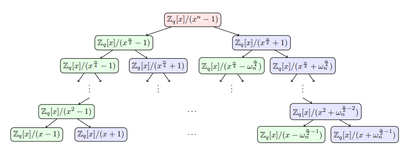
Similarly, for PWC, the modulus polynomial \(x^n - 1\) admits a similar CRT isomorphism map:

From the ring-isomorphism decomposition above, we can already see the rough shape of the butterfly operation. In the next section, we introduce the butterfly operation of the fast Number Theoretic Transform, namely the Cooley-Tukey algorithm, and the butterfly operation of the fast inverse Number Theoretic Transform, namely the Gentleman-Sande algorithm.

CT/GS Butterfly Algorithms

Let \(\varphi\) be a primitive \(2n\)-th root of unity over \(\mathbb{Z}_q\), and let \(\omega := \varphi^2\) be a primitive \(n\)-th root of unity over \(\mathbb{Z}_q\). Here \(n\) is exactly a power of two, so the recursion can proceed completely.

The key properties of the fast Fourier transform are:

\[\varphi^{k+2n} = \varphi^{k} \\ \varphi^{k+n} = -\varphi^{k}\]

To unify notation, let the number theoretic transform for positive wrapped convolution be denoted by \(\textsf{NTT}^{+}\), and the number theoretic transform for negacyclic convolution be denoted by \(\textsf{NTT}^{-}\). Since \(\omega := \varphi^2\), both can be written uniformly in terms of \(\varphi\):

\[\begin{cases} \textsf{NTT}^{+}: & \hat{\mathbf{a}}_j = \sum_{i=0}^{n-1} \varphi^{i \cdot 2j} \mathbf{a}_i \pmod q, & j = 0, 1, 2, \dots, n-1 \\ \textsf{NTT}^{-}: & \hat{\mathbf{a}}_j = \sum_{i=0}^{n-1} \varphi^{i \cdot (2j + 1)} \mathbf{a}_i \pmod q, & j = 0, 1, 2, \dots, n-1 \\ \end{cases}\]

We only need to consider the negacyclic convolution case below, because the corresponding positive wrapped convolution transform can be obtained easily through coefficient reconstruction \(\mathbf{b}_i :=\varphi^{-i} \cdot \mathbf{a}_i\).

Fast-NTT: Cooley-Tukey Algorithm

Consider the first ring-isomorphism step below:

\[\begin{aligned} \hat{\boldsymbol{a}}_j & =\sum_{i=0}^{n-1} \varphi^{2 i j+i} a_i \bmod q \\ & = \left[ \sum_{i=0}^{n / 2-1} \varphi^{4 i j+2 i} a_{2 i}+\sum_{i=0}^{n / 2-1} \varphi^{4 i j+2 j+2 i+1} a_{2 i+1} \right] \bmod q \\ & = \left[ \sum_{i=0}^{n / 2-1} \varphi^{4 i j+2 i} a_{2 i}+\varphi^{2 j+1} \sum_{i=0}^{n / 2-1} \varphi^{4 i j+2 i} a_{2 i+1} \right]\bmod q \end{aligned}\]

Now consider the coefficient with \(J = j + n/2 > n/2\):

\[\hat{\boldsymbol{a}}_{J} = \hat{\boldsymbol{a}}_{j+n / 2}=\sum_{i=0}^{n / 2-1} \varphi^{4 i j+2 i} a_{2 i}-\varphi^{2 j+1} \sum_{i=0}^{n / 2-1} \varphi^{4 i j+2 i} a_{2 i+1} \quad \bmod q, j \in [0,n/2 - 1]\]

This gives some reusable intermediate quantities. Let \(A_j=\sum_{i=0}^{n / 2-1} \varphi^{4 i j+2 i} a_{2 i}\) and \(B_j=\sum_{i=0}^{n / 2-1} \varphi^{4 i j+2 i} a_{2 i+1}\). From the decomposition, we obtain:

\[\begin{cases} \text{Former}: & \hat{\boldsymbol{a}}_j & =A_j+\varphi^{2 j+1} B_j \quad \bmod q \\ \text{Latter}: &\hat{\boldsymbol{a}}_{j+n / 2} & =A_j-\varphi^{2 j+1} B_j \quad \bmod q \end{cases}\]

The coefficients \(A_j, B_j\) can themselves be computed by \(n/2\)-point NTTs. Define:

\[\begin{cases} \mathbf{a}^{(0)} = (a_0, a_2, \ldots, a_{n-2}) \\ \mathbf{a}^{(1)} = (a_1, a_3, \ldots, a_{n-1}) \end{cases}\]

Let \(\omega = \varphi^2\) be a primitive \(2 \cdot \left( \frac{n}{2} \right)\)-th root of unity. We have:

\[\begin{cases} \mathbf{A} = \textsf{NTT}_{n/2}^{\omega}(\mathbf{a}^{(0)}), & A_j=\sum_{i=0}^{n / 2-1} \varphi^{4 i j+2 i} a_{2 i} = \sum_{i=0}^{n / 2-1} \omega^{2ij+i} a_{2 i} \\ \mathbf{B} = \textsf{NTT}_{n/2}^{\omega}(\mathbf{a}^{(1)}), & B_j=\sum_{i=0}^{n / 2-1} \varphi^{4 i j+2 i} a_{2 i + 1} = \sum_{i=0}^{n / 2-1} \omega^{2ij+i} a_{2 i + 1} \end{cases}\]

We recurse in this way until the NTT coefficients can be computed in constant time.

For the standard NTT for positive wrapped convolution, the recursive structure is the same. One only needs to replace \(\varphi^{2j+1}\) above by \(\omega^j\) and replace the subproblem root by \(\omega^2\).

Fast-iNTT: Gentleman-Sande Algorithm

Recall that the inverse NTT is computed as follows:

\[\begin{aligned} \mathbf{a}_j &= \frac{1}{n} \cdot \varphi^{-j} \sum_{i=0}^{n-1} \varphi^{-(2ij)} \hat{\mathbf{a}}_i \bmod q \\ & = \frac{1}{n} \sum_{i=0}^{n-1} \varphi^{-j(2i + 1)} \hat{\mathbf{a}}_i \pmod q \\ \end{aligned}\]

The fast computation of the inverse NTT is decomposed as:

\[\begin{aligned} \mathbf{a}_j & = \frac{1}{n} \sum_{i=0}^{n-1} \varphi^{-j (2i + 1)} \hat{\mathbf{a}}_i \bmod q \\ & = \frac{1}{n} \cdot \varphi^{-j} \left[ \sum_{i=0}^{n / 2-1} \varphi^{-2ij} \hat{\mathbf{a}}_i +\sum_{i=n/2}^{n - 1} \varphi^{-2ij} \hat{\mathbf{a}}_i \right] \bmod q \\ & = \frac{1}{n} \cdot \varphi^{-j} \left[ \sum_{i=0}^{n / 2-1} \varphi^{-2ij} \hat{\mathbf{a}}_i +\sum_{i=0}^{n/2 - 1} \varphi^{-2(i + n/2)j} \hat{\mathbf{a}}_{i + n/2} \right] \bmod q \\ & = \frac{1}{n} \cdot \varphi^{-j} \left[ \sum_{i=0}^{n / 2-1} \varphi^{-2ij} \hat{\mathbf{a}}_{i} + (-1)^j \sum_{i=0}^{n/2 - 1} \varphi^{-2ij} \hat{\mathbf{a}}_{i + n/2} \right] \bmod q \\ & = \frac{1}{n} \cdot \varphi^{-j} \left[ \sum_{i=0}^{n / 2-1} \varphi^{-2ij} \left( \hat{\mathbf{a}}_{i} + (-1)^j \hat{\mathbf{a}}_{i + n/2} \right) \right] \bmod q \\ \end{aligned}\]

The even and odd coefficients can be separated as follows:

\[\begin{cases} \mathbf{a}_{2k} & = \frac{1}{n} \cdot \varphi^{-2k} \left[ \sum_{i=0}^{n / 2-1} \left( \varphi^{-4ki} \left( \hat{\mathbf{a}}_{i}+ \hat{\mathbf{a}}_{i + n/2} \right) \right) \right] \bmod q \\ \mathbf{a}_{2k+1} & = \frac{1}{n} \cdot \varphi^{-2k - 1} \left[ \sum_{i=0}^{n / 2-1} \left( \varphi^{-2i(2k + 1)} \left( \hat{\mathbf{a}}_{i} - \hat{\mathbf{a}}_{i + n/2} \right) \right) \right] \bmod q \\ \end{cases}\]

Next, we analyze the recursive formula from two perspectives.

Inverting the CT Transform

The Gentleman-Sande inverse transform can be obtained directly by inverting the butterfly formula from the Cooley-Tukey forward transform in the previous section. Recall the CT forward transform in the negacyclic convolution setting. Split the input coefficients by even and odd indices:

\[\begin{cases} \mathbf{a}^{(0)} = (a_0, a_2, \ldots, a_{n-2}) \\ \mathbf{a}^{(1)} = (a_1, a_3, \ldots, a_{n-1}) \end{cases}\]

Let \(\omega = \varphi^2\). Then \(\omega\) is the primitive \(n\)-th root of unity needed for the length \(n/2\) negacyclic subproblem; in other words, it plays the role of a primitive \(2\cdot(n/2)\)-th root of unity inside the subproblem. Write:

\[\begin{cases} \mathbf{E} = \textsf{NTT}_{n/2}^{\omega}(\mathbf{a}^{(0)}), & E_j=\sum_{i=0}^{n / 2-1} \varphi^{4 i j+2 i} a_{2 i} = \sum_{i=0}^{n / 2-1} \omega^{2 i j+i} a_{2 i} \\ \mathbf{O} = \textsf{NTT}_{n/2}^{\omega}(\mathbf{a}^{(1)}), & O_j=\sum_{i=0}^{n / 2-1} \varphi^{4 i j+2 i} a_{2 i+1} = \sum_{i=0}^{n / 2-1} \omega^{2 i j+i} a_{2 i+1} \end{cases}\]

The CT butterfly gives:

\[\begin{cases} \hat{\mathbf{a}}_j = E_j + \varphi^{2j+1} O_j, & j = 0, \ldots, \frac{n}{2}-1 \\ \hat{\mathbf{a}}_{j+n/2} = E_j - \varphi^{2j+1} O_j, & j = 0, \ldots, \frac{n}{2}-1 \end{cases}\]

The GS inverse transform inverts this linear system layer by layer. Given the evaluation vector \(\hat{\mathbf{a}}\) at the current layer, first pair the upper and lower halves to recover two length \(n/2\) subproblem evaluation vectors:

\[\begin{cases} E_j = \frac{1}{2}\left(\hat{\mathbf{a}}_j + \hat{\mathbf{a}}_{j+n/2}\right), & j = 0, \ldots, \frac{n}{2}-1 \\ O_j = \frac{1}{2\varphi^{2j+1}}\left(\hat{\mathbf{a}}_j - \hat{\mathbf{a}}_{j+n/2}\right), & j = 0, \ldots, \frac{n}{2}-1 \end{cases}\]

Then recursively apply length \(n/2\) inverse transforms to \(\mathbf{E}\) and \(\mathbf{O}\):

\[\begin{cases} \mathbf{a}^{(0)} = \textsf{iNTT}_{n/2}^{\omega}(\mathbf{E}) \\ \mathbf{a}^{(1)} = \textsf{iNTT}_{n/2}^{\omega}(\mathbf{O}) \end{cases}\]

Finally, interleave the coefficients of the two subproblems:

\[\begin{cases} a_{2r} = a^{(0)}_r, & r = 0, \ldots, \frac{n}{2}-1 \\ a_{2r+1} = a^{(1)}_r, & r = 0, \ldots, \frac{n}{2}-1 \end{cases}\]

The recursion terminates at \(n=1\), where the input evaluation vector is already the coefficient vector. Since each butterfly layer multiplies by \(\frac{1}{2}\) and there are \(\log_2 n\) layers in total, the total scaling factor is:

\[\left(\frac{1}{2}\right)^{\log_2 n} = \frac{1}{n}\]

This exactly matches the normalization factor \(\frac{1}{n}\) in the iNTT definition. Therefore, an implementation can use \(2^{-1} \bmod q\) at each layer, without multiplying by \(n^{-1}\) again after the recursion ends.

Deriving the Standard GS Transform

We can derive the recursion directly from the definition of \(\textsf{iNTT}^{\varphi}\). Let the input evaluation vector at the current layer be \(\hat{\mathbf{a}}=(\hat{\mathbf{a}}_0,\ldots,\hat{\mathbf{a}}_{n-1})\), and let the output coefficient vector be \(\mathbf{a}=(\mathbf{a}_0,\ldots,\mathbf{a}_{n-1})\). By definition:

\[\mathbf{a}_j = \frac{1}{n}\sum_{i=0}^{n-1}\varphi^{-j(2i+1)}\hat{\mathbf{a}}_i \pmod q\]

Split the output index \(j\) into even and odd cases. For even index \(j=2k\):

\[\begin{aligned} \mathbf{a}_{2k} &= \frac{1}{n}\sum_{i=0}^{n-1}\varphi^{-2k(2i+1)}\hat{\mathbf{a}}_i \\ &= \frac{1}{n}\varphi^{-2k}\sum_{i=0}^{n-1}\varphi^{-4ki}\hat{\mathbf{a}}_i \\ &= \frac{1}{n}\varphi^{-2k}\sum_{i=0}^{n/2-1} \left(\varphi^{-4ki}\hat{\mathbf{a}}_i+\varphi^{-4k(i+n/2)}\hat{\mathbf{a}}_{i+n/2}\right) \\ &= \frac{1}{n}\varphi^{-2k}\sum_{i=0}^{n/2-1} \varphi^{-4ki}\left(\hat{\mathbf{a}}_i+\hat{\mathbf{a}}_{i+n/2}\right) \end{aligned}\]

The last step uses \(\varphi^{-4k(i+n/2)}=\varphi^{-4ki}\varphi^{-2kn}=\varphi^{-4ki}\).

For odd index \(j=2k+1\):

\[\begin{aligned} \mathbf{a}_{2k+1} &= \frac{1}{n}\sum_{i=0}^{n-1}\varphi^{-(2k+1)(2i+1)}\hat{\mathbf{a}}_i \\ &= \frac{1}{n}\varphi^{-(2k+1)}\sum_{i=0}^{n-1}\varphi^{-2(2k+1)i}\hat{\mathbf{a}}_i \\ &= \frac{1}{n}\varphi^{-(2k+1)}\sum_{i=0}^{n/2-1} \left(\varphi^{-2(2k+1)i}\hat{\mathbf{a}}_i+\varphi^{-2(2k+1)(i+n/2)}\hat{\mathbf{a}}_{i+n/2}\right) \\ &= \frac{1}{n}\varphi^{-(2k+1)}\sum_{i=0}^{n/2-1} \varphi^{-2(2k+1)i}\left(\hat{\mathbf{a}}_i-\hat{\mathbf{a}}_{i+n/2}\right) \end{aligned}\]

The last step uses \(\varphi^{-2(2k+1)(i+n/2)}=-\varphi^{-2(2k+1)i}\).

Now let the primitive root of the subproblem be \(\omega=\varphi^2\), and define two new evaluation vectors of length \(n/2\):

\[\begin{cases} E_i = \frac{1}{2}\left(\hat{\mathbf{a}}_i+\hat{\mathbf{a}}_{i+n/2}\right), \\ O_i = \frac{1}{2}\varphi^{-(2i+1)}\left(\hat{\mathbf{a}}_i-\hat{\mathbf{a}}_{i+n/2}\right), \end{cases} \quad i=0,\ldots,\frac{n}{2}-1\]

We can observe that the two length \(n/2\) recursive subproblems \(\textsf{iNTT}^{\omega}\) give:

\[\begin{aligned} \textsf{iNTT}_{n/2}^{\omega}(\mathbf{E})_k &= \frac{2}{n}\sum_{i=0}^{n/2-1}\omega^{-k(2i+1)}E_i \\ &= \frac{1}{n}\varphi^{-2k}\sum_{i=0}^{n/2-1} \varphi^{-4ki}\left(\hat{\mathbf{a}}_i+\hat{\mathbf{a}}_{i+n/2}\right) \\ &= \mathbf{a}_{2k}, \end{aligned}\]

and:

\[\begin{aligned} \textsf{iNTT}_{n/2}^{\omega}(\mathbf{O})_k &= \frac{2}{n}\sum_{i=0}^{n/2-1}\omega^{-k(2i+1)}O_i \\ &= \frac{1}{n}\sum_{i=0}^{n/2-1} \varphi^{-2k(2i+1)}\varphi^{-(2i+1)} \left(\hat{\mathbf{a}}_i-\hat{\mathbf{a}}_{i+n/2}\right) \\ &= \frac{1}{n}\varphi^{-(2k+1)}\sum_{i=0}^{n/2-1} \varphi^{-2(2k+1)i}\left(\hat{\mathbf{a}}_i-\hat{\mathbf{a}}_{i+n/2}\right) \\ &= \mathbf{a}_{2k+1}. \end{aligned}\]

Therefore, directly from the iNTT formula, we obtain the recurrence:

\[\begin{cases} (\mathbf{a}_0,\mathbf{a}_2,\ldots,\mathbf{a}_{n-2}) = \textsf{iNTT}_{n/2}^{\varphi^2}(\mathbf{E}) \\ (\mathbf{a}_1,\mathbf{a}_3,\ldots,\mathbf{a}_{n-1}) = \textsf{iNTT}_{n/2}^{\varphi^2}(\mathbf{O}) \end{cases}\]

The core of the recursion is computing the vectors \(\mathbf{E}\) and \(\mathbf{O}\):

\[\begin{cases} E_i \leftarrow 2^{-1}(\hat{\mathbf{a}}_i+\hat{\mathbf{a}}_{i+n/2}) \pmod q \\ O_i \leftarrow 2^{-1}(\hat{\mathbf{a}}_i-\hat{\mathbf{a}}_{i+n/2})\cdot(\varphi^{2i+1})^{-1} \pmod q \end{cases}\]

Notice that the final step interleaves the results of the two recursive subproblems by even and odd indices. The recursive version here does not require bit reversal, and it also does not require an additional multiplication by \(n^{-1}\) at the end, because the \(2^{-1}\) factor at each layer already accumulates to the normalization factor \(n^{-1}\) in the inverse NTT definition.

For the iNTT of positive wrapped convolution, the recursive structure is the same. One only needs to replace \(\varphi^{2j+1}\) by \(\omega^j\) and replace the subproblem root by \(\omega^2\):

\[\begin{cases} E_j = \frac{1}{2}\left(\hat{\mathbf{a}}_j + \hat{\mathbf{a}}_{j+n/2}\right) \\ O_j = \frac{1}{2\omega^j}\left(\hat{\mathbf{a}}_j - \hat{\mathbf{a}}_{j+n/2}\right) \end{cases}\]

Non-Recursive Iterative Butterfly Algorithms

The recursive CT/GS algorithms are best suited for understanding where the formulas come from, but practical implementations usually unroll the recursion into an iterative butterfly network. The essence of recursive CT is that it repeatedly splits subproblems according to the parity of the input index: the first layer looks at the least significant bit, the second layer at the next bit, and so on until the most significant bit. Therefore, the input order at the leaves of the recursion tree is exactly the bit-reversal permutation (BO order) of the original indices. Let \(\operatorname{brv}_{\ell}(i)\) denote the integer obtained by reversing the \(\ell=\log_2 n\) bits of \(i\). For example, when \(n=8\):

\[(0,1,2,3,4,5,6,7) \mapsto (0,4,2,6,1,5,3,7)\]

Expanding in three bits, the correspondence is:

\[\begin{cases} 000_2 \mapsto 000_2, & 0 \mapsto 0 \\ 001_2 \mapsto 100_2, & 1 \mapsto 4 \\ 010_2 \mapsto 010_2, & 2 \mapsto 2 \\ 011_2 \mapsto 110_2, & 3 \mapsto 6 \\ 100_2 \mapsto 001_2, & 4 \mapsto 1 \\ 101_2 \mapsto 101_2, & 5 \mapsto 5 \\ 110_2 \mapsto 011_2, & 6 \mapsto 3 \\ 111_2 \mapsto 111_2, & 7 \mapsto 7 \end{cases}\]

For \(n = 8\), suppose the input coefficient vector is in natural order (NO): \((a_0,a_1,a_2,a_3,a_4,a_5,a_6,a_7)\). The final output vector is not in natural order, but in BO order: \((\hat a_0 \mid \hat a_4 \mid \hat a_2 \mid \hat a_6 \mid \hat a_1 \mid \hat a_5 \mid \hat a_3 \mid \hat a_7)\). The detailed permutation during the CT operation is:

\[\begin{aligned} &\textbf{Cooley-Tukey:} \text{NO} \to \text{BO} \\[2mm] &(a_0,a_1,a_2,a_3,a_4,a_5,a_6,a_7) \\ &\xrightarrow{\text{split by bit }0} (a_0,a_2,a_4,a_6 \mid a_1,a_3,a_5,a_7) \\ &\xrightarrow{\text{split by bit }1} (a_0,a_4 \mid a_2,a_6 \mid a_1,a_5 \mid a_3,a_7) \\ &\xrightarrow{\text{split by bit }2} (a_0 \mid a_4 \mid a_2 \mid a_6 \mid a_1 \mid a_5 \mid a_3 \mid a_7) \\ &\qquad = (\hat{a}_{\operatorname{brv}_3(0)},\hat{a}_{\operatorname{brv}_3(1)},\dots,\hat{a}_{\operatorname{brv}_3(7)}) \end{aligned}\]

This is exactly the left-to-right order of the leaf nodes after CT recurses to the bottom. The permutation has order two, so applying the same permutation again flips the sequence from BO order back to normal NO order. In fact:

1. If the input is in BO order, CT butterfly operations produce NO order.
2. If the input is in NO order, CT butterfly operations produce BO order.

Returning to the Gentleman-Sande butterfly operation, the permutation is exactly the same from the output perspective. In short, if we want to obtain the normal NO sequence, we need to permute the result vector back from BO order at the end. After clarifying the ordering, we continue to analyze the iterative form of the Fast NTT algorithm.

Non-Recursive Cooley-Tukey NTT

For the standard NTT for positive wrapped convolution, let \(\omega\) be a primitive \(n\)-th root of unity. The iterative CT algorithm first reorders the input coefficient vector in bit-reversal order, then starts from small blocks of length \(m=2\) and merges upward, doubling \(m\) layer by layer until \(m=n\). Within each block of length \(m\), the local primitive \(m\)-th root of unity is:

\[\omega_m = \omega^{n/m}\]

For block position \(j=0,\ldots,m/2-1\), the CT butterfly is:

\[\begin{cases} u = a_{\text{start}+j} \\ v = \omega_m^j \cdot a_{\text{start}+j+m/2} \end{cases} \implies \begin{cases} a_{\text{start}+j} \leftarrow u+v \pmod q \\ a_{\text{start}+j+m/2} \leftarrow u-v \pmod q \end{cases}\]

For \(\textsf{NTT}^{\varphi}\) in negacyclic convolution, let \(\varphi\) be a primitive \(2n\)-th root of unity. In a local subproblem of length \(m\), the corresponding primitive \(2m\)-th root of unity is:

\[\varphi_m = \varphi^{n/m}\]

The CT butterfly in the negacyclic version only needs to replace the twiddle factor \(\omega_m^j\) in the standard NTT by the odd power:

\[\varphi_m^{2j+1}\]

That is:

\[\begin{cases} u = a_{\text{start}+j} \\ v = \varphi_m^{2j+1} \cdot a_{\text{start}+j+m/2} \end{cases} \implies \begin{cases} a_{\text{start}+j} \leftarrow u+v \pmod q \\ a_{\text{start}+j+m/2} \leftarrow u-v \pmod q \end{cases}\]

Non-Recursive Gentleman-Sande iNTT

The GS inverse transform can be viewed as running the CT butterfly network backward. CT merges from small blocks into larger blocks, so GS splits from large blocks into smaller blocks. For the iNTT of standard positive wrapped convolution, define within a block of length \(m\):

\[\omega_m = \omega^{n/m}\]

The GS butterfly is:

\[\begin{cases} u = a_{\text{start}+j} \\ v = a_{\text{start}+j+m/2} \end{cases} \implies \begin{cases} a_{\text{start}+j} \leftarrow \frac{u+v}{2} \pmod q \\ a_{\text{start}+j+m/2} \leftarrow \frac{u-v}{2\omega_m^j} \pmod q \end{cases}\]

Here \(\frac{1}{2}\) is placed inside each butterfly layer. Since there are \(\log_2 n\) layers in total, the overall scaling is \(1/n\). Another common form omits the factor \(\frac{1}{2}\) at each layer and instead multiplies by \(n^{-1}\) at the end; the two forms are equivalent. The current code uses the former form, so no additional multiplication by \(n^{-1}\) is needed at the end. After each GS layer, the data still follows the grouping order of recursive splitting. After all layers have been executed, the coefficients are in bit-reversal order, so one more bit reversal is needed to return to natural order.

For \(\textsf{iNTT}^{\varphi}\) in negacyclic convolution, similarly let the local root be:

\[\varphi_m = \varphi^{n/m}\]

Then replace \(\omega_m^j\) by \(\varphi_m^{2j+1}\):

\[\begin{cases} a_{\text{start}+j} \leftarrow 2^{-1}(u+v) \pmod q \\ a_{\text{start}+j+m/2} \leftarrow 2^{-1}(u-v)(\varphi_m^{2j+1})^{-1} \pmod q \end{cases}\]